What to do if the supplier convinces you to purchase expensive control valves, while hiding their types and characteristics. In this article we will briefly look at the types and characteristics of control valves. It is worth noting that there are a huge number of models from different manufacturers on the market, so even if you have extensive experience in operating pipeline systems, it is better to entrust the choice of specific equipment to specialists with extensive installation experience. Our specialists will select equipment for engineering units while maintaining operating parameters and stable operation after installation! Let's take a closer look at what control valves there are.
What is it and what is it for?
A control valve is one of the types of control fittings, the main function of which, as you can guess from the name, is to regulate the movement of contents in the pipeline. This is done by changing the pressure and flow rate of the medium entering through the through hole of the fittings.
Along with it, a shut-off and control valve is used, which not only has the function of automatically changing the flow rate, but is also capable of completely stopping the flow circulation.
The functions of control and shut-off valves are combined in a shut-off and control valve.
Construction company LLC "STM"
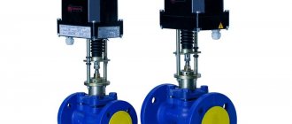
A control valve is used as one of the units of pipeline fittings for heating and water supply systems. The principle of its operation differs little from valves and taps, since it serves to regulate the flow of the coolant medium. In the vast majority of cases it is water. Controlling its flow using a valve comes down to regulating pressure and flow. Most often, steel shut-off and control valves are used for hot water, although metal-plastic ones are also found.
As a rule, for manual adjustment, shut-off and control valves are used, which are capable of blocking the flow not only partially, but also completely. In other cases, automatic valves with various types of drives have been used:
- electromagnetic;
- electrical;
- hydraulic;
- pneumatic.
Types of drives powered by electrical energy are used more often, since they do not require laying special lines and installing compressor equipment.
How control valves are attached
To install control valves into a pipeline, various fastening methods are used that can ensure high tightness of the connection at a given fluid pressure. Thus, the fitting method can be used, but where high pressures are involved, flange, coupling or welded methods are more often used, as well as a pin connection, in which the fittings are screwed directly into the body of the apparatus connected to the pipeline.
The welding method is used exclusively for steel control valves.
Dividing valves according to flow direction
The configuration and number of valve connections differs depending on how it is intended to conduct water flow. For direct, a conventional straight-through valve is used. If you need to turn the flow at a right angle, then an angle control valve is used, and if you need to mix two flows, then a three-way type of this valve is installed. Plumbers call such valves faucets, since these fittings have two inlets and one outlet.
Valve design
Control valves can be implemented in different ways. There are several types of valve designs:
- membrane;
- cellular;
- plunger
Plunger valves are divided into single- and double-seat valves. The former are used for small pipeline sections, the latter for large pipeline clearances. In the first situation, it does not matter whether the plunger is balanced or not. In the second case, it is preferable to use balanced plungers, which is ensured by the double-seat valve design.
Where it is necessary to achieve silent operation of the crane, a cellular design is used, which consists in the fact that the control element is made in the form of a cylinder with a cavity. This cylinder moves inside the perforated cage, thereby regulating the force of fluid flow.
Diaphragm valves are used where fully automatic flow control is needed. Often the design of such valves has feedback, with which you can regulate the flow of water without using third-party drives. This type of fittings is convenient to use where you can set the required pressure value in the area once. The valve will support it without outside intervention.
Controls and technical characteristics
Manual control has now been replaced by modern methods of controlling control valves, based on the use of various types of drives and combinations of sensors that detect the slightest changes in the state of the pipeline contents.
According to the purpose and conditions of use, the following types of control are used:
- hydraulic;
- electrical;
- electromagnetic.
- pneumatic.
valves are:
- capacity in Kv;
- diameter DN;
- nominal pressure rating;
- working temperature.
The specified characteristics can be found in the technical documentation supplied by the manufacturers to the product. The features inherent in this type of control valves are a quick response to changes in environmental characteristics and reliable tightness.
Connection type
Depending on the type of connection to network pipes, control valves are:
- welded;
- flanged;
- fitting
- coupling;
- tsapkovymi.
Welded fittings (for welding) are produced only in a steel casing. This type of connection is the most reliable, but has a high execution price and is limited in maintainability. Used in industrial networks.
Flange products have found the widest application in all major highways with various environments. In household communications, control valves are connected through threaded connections on couplings.
Device
Let us consider, using the example of a flanged single-seat control valve, the design of this type of valve.
The device consists of a cast body B, in which a passage hole called seat V is placed. A plunger T is lowered into it, fixed on a rod S moving up and down. Flanges F are welded to the body, through which the unit is connected to the pipeline. The sealing unit P serves to seal the entire device.
Principle of operation
The essence of the operation of a control valve is to move a plunger or other type of valve under the pressure of a moving medium. When the shut-off element blocks part of the orifice, the flow of liquid or gas passing through the valve is reduced. Complete closure of the valve causes the flow to be blocked and the pressure in the system to drop to zero.
Based on their operating principle, control devices are divided into those that block, mix or separate the flow of the working medium. Shutting valves include two-way valves, and mixing valves include three- and four-way valves.
Design and principle of operation [edit | edit code ]
The explanatory figure on the right shows a sectional view of a simple straight-through single-seat control valve. Where:
- B
—valve body; - F
- flange for connecting fittings to the pipeline. - P
- sealing unit, ensuring the tightness of the fittings in relation to the external environment; - S
- valve stem transmitting translational force from a mechanized or manual drive
to a valve
consisting of
a plunger
and
seat
; - T
-
plunger
, with its profile determines the control characteristics of the valve; - V
-
seat
, an element that ensures
the plunger
in the extreme closed position.
The force from the drive is transmitted via a rod to the valve, which consists of a plunger and a seat. The plunger blocks part of the flow area, which leads to a decrease in flow through the valve. According to Bernoulli's law, the flow velocity of the medium increases, and the static pressure in the pipe decreases. When completely closed, the plunger sits in the seat, the flow is blocked, and if the valve is completely sealed, the pressure after the valve will be zero [1].
Types and designs
Depending on the functions for changing the direction of flow, the devices we are considering are:
- passageways that do not change the direction of the medium; Globe valves are installed in pipeline sections without bends;
- angular, shifting the medium at a right angle;
- mixing, mixing two types of flows with different states into one.
According to their design features, control valves are:
- saddle;
- cellular;
- membrane;
- spool types.
Differences
In saddle devices, the locking element is made in the form of a rod, disc or needle plunger. In small cross-section pipes, single-seat fittings are installed; in networks with a diameter of up to 300 mm and a pressure of up to 6.5 MPa, double-seated fittings are installed, which have better tightness and a more balanced plunger.
A feature of cage-type structures is their shutter, made in the form of a cylindrical piston located in the cage. This design reduces noise and vibration when the valve is turned on.
The difference between membrane fittings is the limitations in control methods: their devices are equipped only with pneumatic or hydraulic actuators. The membrane serves as a shutter in them.
In spool valves, the flow level is regulated by turning the valve, that is, the spool, as a result of which the flow hole is partially opened or closed. The mechanism of operation of this fitting is in many ways similar to the operation of an ordinary ball valve.
Types of control valves
Depending on the design of the regulatory bodies, the fittings are divided into:
- saddle;
- cellular;
- membrane;
- spool valve
The seat valve, in turn, can have 1 or 2 seats. Single-seat fittings have one through hole; such structures are installed on pipelines of small diameters (up to 150 mm). The 2-seat valve has the advantage of a balanced plunger; it can be used in systems with pressures up to 6.5 MPa and diameters up to 300 mm . The shut-off plunger can be made in a rod, disc or needle configuration.
Diagram of cage valve design
In cage-type fittings, the gate has the shape of a hollow cylinder moving inside the hole - a cage, which simultaneously acts as a guide device and a passage unit. The cylinder itself has radial perforation, due to which the pressure in the pipeline is adjusted. The design features of the cage fittings ensure a minimum level of noise and vibration during valve operation.
Unlike seat and cage valves, which can be equipped with a manual drive, diaphragm valves are produced exclusively with pneumatic or hydraulic drives. The shutter in it is an elastic rubber membrane (less commonly, a fluoroplastic membrane). The drive can be remote or built-in.
Since the flexibility of the membrane can cause errors in pressure regulation, the valve is equipped with an additional unit - a positioner that controls the spatial position of the rod connecting the membrane to the drive. The advantages of membrane structures include the resistance of the rubber seal to chemically aggressive environments and corrosion, which allows the use of such fittings on pipelines of the chemical industry and lines transporting petroleum products.
Diaphragm valve design
The spool valve regulates the pressure level of the working medium by rotating the shutter (spool) to a certain angle, which leads to partial opening or closing of the passage hole. According to the principle of operation, such fittings are similar to conventional ball valves; they are most often used in the energy industry.
The advantage of spool valves is the need to apply minimal effort when controlling the valve, since the fluid pressure in the through hole has virtually no resistance to the movement of the shut-off element. However, such designs are not a way to ensure complete tightness of cutting off the working medium when the seat is closed, so they are practically not used on pipelines with high pressure.
Marking
Technical requirements for control valves are given in the regulatory document GOST No. 12893 “Single-seat, double-seat and cage control valves”. According to the provisions of GOST, all valves have a unified marking type 21ch10nzh , in which:
- 21 – type of fittings (pressure regulators have a numerical nomenclature of 21 and 19);
- h – body material (h – cast iron, s – carbon steel, b – brass or bronze, tn – titanium, p – plastic);
- 10 – type of drive (in this case – mechanical, 6 – pneumatic, 7 – hydraulic);
- NZ – material for manufacturing sealing surfaces, stainless steel.
The main domestic manufacturer of valves is the Avangard company (Stary Oskol Valve Plant). Among foreign companies, we note the companies Dafnoss (Denmark), Bugatti (Italy) and FAR (Italy).
Advantages and disadvantages
The advantages of control valves that ensure their popularity are:
- the ability to regulate the flow of contents in the pipeline in various ranges, how they differ from devices such as a valve;
- ease of management and operation;
- resistance to various types of working environment;
- possibility of choice depending on the purpose and conditions of use.
The disadvantages include
- the high price of regulators with electric drives and significant costs for monitoring and maintenance;
- overheating of the electric motor during prolonged operation;
- significant hydraulic resistance;
- a certain amount of leakage, in contrast to shut-off devices, allowed by GOST.
Linear operating flow characteristic of the valve
The RLV-S control valves, designed for piping heating devices, as well as ASV-I, USV-I, MSV-I, MSV-F (d
>
250 mm), MSV-F Plus (сi > 250 mm) have a linear operating flow characteristic ) (Fig. 3.7), installed on risers, instrument branches, highways, etc. A distinctive feature of large diameter valves MSV-F (
D
= 250...400) and MSV-F Plus
(d =
250...400) is that that to ensure the stability of their operation, the shutter is made hollow with rectangular windows (see Fig. 3.5,a).
For valves with a linear flow characteristic, under ideal conditions, the relationship between water flow and rod stroke is observed:
AV AG /CH1CHH
V~
=
~ R ~= T.
' <313>
'100 «100 «i 00
Where V100 and G100 are the maximum possible respectively volumetric, m3/h, or mass, kg/h, water flow through the valve; hm
is
the total displacement (stroke) of the valve stem, mm; c is the proportionality coefficient.
-V
| MSV-I |
| RLV-S straight |
RLV-S corner
| USV-I |
| ASV-I |
| MSV-F (s/ = 250..400) |
| MSV-F Plus (s/= 250..400) |
Rice. 3.7. Control valves with linear flow characteristic
| 0 0,1 0,2 0,3 0,4 0,5 0,6 0,7 0,8 0,9 1,0 H/HIDo Rice. 3.8. Linear operating flow characteristic of the valve |
Dependence (3.13) is valid with the full external authority of the valve a+ = 1 (all available pressure of the regulated section is lost in the control hole). Over the entire range of stroke of the rod, its relative movement AMg0 leads to an equal relative change in flow rate AV / Vm .
However, this proportion is violated as the authority of the valve decreases.
The lower the authority, the greater the curvature of the flow characteristic, i.e., the greater the misalignment of the system. In this case, the proportionality coefficient c
becomes a variable value.
In real conditions, when choosing a valve without taking into account authority, its flow characteristic differs from the design one. So, if the valve shutter is set to position AMgsh0 = 0.6, then the excess flow rate at A+ =
0.3 is 100(0.8 - 0.6)/0.6 = 33% (see dotted lines in Fig. 3.8). Consequently, this valve will cause a redistribution of flows in the system and will not ensure efficient operation of the heat exchange equipment. It must be additionally configured when setting up the system. However, this can be avoided by choosing a valve with authority in mind.
The flow characteristics of the valve may differ from ideal ones, and regulation occurs according to a deformed linear law even with external authority a = 1. To better understand this statement, it is necessary to conditionally divide the valve resistance into two components: the resistance of the control hole under the valve shutter and the resistance of the rest of the passage channel coolant inside the valve body. Ideal conditions will occur when the second component is equal to zero. The hydraulic resistance of the valve body can be interpreted as the corresponding resistance of the pipeline section, which creates the initial deformation of the ideal characteristic. The approach used in hydraulics is called the equivalent length method. Therefore, the hydraulic characteristics of control valves (except for valves with zero resistance in the maximum open position) provided by manufacturers already have a distortion of the ideal control law, which is characterized by basic authority. A
external authority contributes to further deformation of the consumption characteristics.
The real distortion of the valve flow characteristic occurs under the influence of the full external authority a , which
A+=aba,
(3.14)
Where is the basic authority of the valve; a is the external authority of the valve.
Current system design practice often takes the initial (baseline) valve flow characteristic provided by the manufacturer as a starting point for further determination of its deformation under the influence of an external authority. However, the underlying distortion of this characteristic is different for each valve, making generalization (determining the recommended external authority range) for hydraulic calculations difficult. An example would be various designs of valve bodies: with a stem perpendicular to the flow, an oblique stem, with a stem inside a ball-shaped valve... It is much more practical to take its ideal characteristic as a starting point for the deformation of the flow characteristics of valves. Then the general equations can be applied to all valve designs.
The influence of the total external authority on the dependence of the relative flow rate on the relative stroke of the valve valve with a linear characteristic has the form [24]:
V 1
| V ‘100 |
———— — ї—— ■ (3.15)
1 - a+ +
(Y /V )
Equation (3.15) in [24] is based on the concept of valve authority, which in its physical essence fully corresponds to the concept of complete external authority considered in this work. Therefore, all equations from [24] are transformed taking into account the distinctions in the accepted terminology.
When designing or setting up a microclimate system, it is necessary to determine the setting of the control valve. To do this, formula (3.15) should be transformed.
A control valve with a threaded spindle is adjusted by rotating it. The speed count starts from the “closed” position. Since the spindle thread is uniform, its full lift is L
|(ω is proportional to the maximum valve setting itax.
E This
parameter is a technical characteristic of the valve and is indicated by the manufacturer. The intermediate position of the spindle
H
corresponds to the intermediate setting
n.
Then, replacing the ratio Mgsh in formula (3.15) with n//?tnax, we obtain the equation for setting the control valve:
» = -,——- ^———— (3.16)
^l-fcoo/r)2
From equation (3.16) it follows that the valve setting depends not only on the flow rate, but also on the overall authority. Under ideal conditions (a+ = 1), equation (3.16) acquires a linear relationship (3.13).
Consumption V100 is determined by calculation. The coincidence of this flow rate with the nominal one is a special case of equation (3.16), when n = itah. This position of the valve does not allow increasing the coolant flow. In this case, it is very unlikely that the pressure drop created by the maximum open control valve at rated flow will be equal to the pressure drop that must be lost across it to balance the circulation ring. Due to the limited choice of hydraulic characteristics of pipelines, hydraulic characteristics of valves in the maximum open position, branched systems and much more, in most cases control valves with preset settings are used. Then the consumption
Rice. 3.9. Pressure distribution in the regulated area: 7 - characteristics of an unregulated pump; 2 - characteristic of the automatic pressure drop regulator; 3 - characteristics of the regulated area under design conditions; 4—characteristics of the regulated section with the control valve fully open; 5 - characteristic of the regulated section without taking into account the resistance of the control valve |
The adjustable section, shown in Fig. 3.9, located between the pressure pulse sampling points of the differential pressure regulator according to the diagram in Fig. 3.3, g. The pressure maintained by this AR regulator is
Is disposable.
The regulated sections are linked along it. The pressure loss of the regulated section, without taking into account the pressure loss at the control valve, is equal to AP
.
Therefore, the pressure loss across the control valve should be D Pv = AP - AP
.
Since the probability of this pressure difference matching the one created by the maximum open valve is too low, the valve has to be adjusted. Then it is advisable to divide the pressure loss on the valve into two terms: pressure loss APVS ,
characterized by the design features of the coolant flow path inside the fully open valve, and pressure loss
ARp,
resulting from movement of the rod from the maximum open position to the required setting position.
Losses APvs, bar, are determined by the maximum valve capacity Kvs ,
(m3/h)/bar0.5, and the nominal flow rate
VN ,
m3/h:
V2
AR
AND
ki
The coolant flow rate U100, m3/h, is determined by the pressure drop across the valve APv, bar, at the nominal flow rate and maximum valve capacity Kvs ,
(m3/h)/bar0.5:
Vm
, = KJAF. (3.18)
| (3.17) |
Then
| KM K: AR |
| AR A R~ |
| (3.19) |
Substituting a+
from equation
(3.14)
and
( Vw [ /VNjl
from equation
(3.19)
In equation
(3.16),
we obtain the equation for tuning a control valve with a linear operating flow characteristic in the form:
| 1 |
| AR Chlr„ |
| AR "6A Ks |
| 1- |
(3.20)
! ARI+AR - |
In this and subsequent equations for setting valves, a modified external authority equation a = APsh
( APvs - AP)
, in which all parameters are calculated based on
the nominal
flow rate, and not on
the Maximum flow rate,
as in equation
(3.12).
This approach is more practical because the nominal flow is a design parameter when designing systems, as opposed to the maximum flow.
Example
2. The control valve
MSV -I
d =
25
mm has a linear flow characteristic. The dependence of the valve capacity on the setting is given in the table provided by the manufacturer.
| Setting position p | 0,2 | 0,5 | 1,0 | 1,5 | 2,0 | 2,5 | 3,0 | 3,2 |
| Valve Capacity Kv, (mугі)/barІ}*' | 0,4 | 1,1 | 1,9 | 2,7 | 3,3 | 3,6 | 3,9 | 4,0 |
| The basic authority of the valve must be determined. |
Solution. The basic valve authority is calculated from the tuning equation (3.16), written as:
A
a -1 Z ^mllL
Uf -tl
U_. —
-^Inf 1 -(n^/n)2
In this example, the external authority a = 1 should be accepted, based on the conditions of the hydraulic test of the valve. Then, substituting the maximum parameters from the last column, and intermediate parameters from any other column of the table, the basic valve authority is found:
1-(4,0/2,7)-
E 1- (3.2/1.5)
For greater accuracy of this parameter, it is necessary to determine its value at each setting and average it. The calculation results are shown in the table.
| Setting position p | 0,2 | 0,5 | 1,0 | 1,5 | 2,0 | 2,5 | 3,0 | 3,2 |
| Basic Valve Authority Ag | 0,39 | 0,31 | 0,37 | 0,34 | 0,30 | 0,37 | 0,38 | — |
Arithmetic mean value a$ =
0,35.
The slight scatter in the tabular data of the basic authority is caused by rounding of the valve capacity and the error in its determination. The valve capacity can be calculated more accurately analytically. To do this, it is necessary to hydraulically test the valve to establish with sufficient reliability the valve capacity at only one setting. The convergence of practical and theoretical calculations is also facilitated by the design improvement of the valve - reducing the backlash of the thread and reducing its pitch on the spindle. In the latter case, the number of settings positions also increases.
Thus, from the considered example 2 it is clear that the flow regulation by this valve with an external authority a = 1 will be carried out according to the flow characteristic displayed by the curve of the total external authority a*
= 0.35 in Fig. 3.8. Further deformation of this characteristic occurs under the influence of external authority.
The current practice of designing microclimate systems, as a rule, does not properly take into account the mutual influence of the basic and external authorities of the control valve on its setting. Manufacturers provide graphs, tables or diagrams corresponding to the basic flow characteristic with an external authority of a = 1. But this is not enough to determine the flow characteristic of the valve in real conditions. With existing approaches, already at the system design stage, conditions can be created for unintended regulation of coolant flows. The resulting redistribution reduces the energy efficiency of the microclimate system, since energy consumption increases, worsens the provision of thermal comfort in the room, and complicates commissioning work.
The result of calculating the valve setting according to the general external authority is similar to the result of the calculation according to kx
or the graphical method provided by the manufacturer in the technical description of the valve. However, this calculation has a significant difference: with the help of a general external authority, it reflects the modification of the regulation process depending on the characteristics of the regulated area, which is discussed in example 3.
Example
3. Design a microclimate system with a branch (riser or horizontal branch).
The closest and only automatic device for stabilizing pressure in the system is a differential pressure regulator installed in an individual heating point according to the diagram in Fig. 3.3, g. The differential pressure it maintains is AP = 0.45
bar.
The resistance of the regulated section without taking into account the pressure loss on the regulating valve is AP = 0.25
bar.
The nominal coolant flow rate in the regulated area is VN = 0.8
m3/h.
It is necessary to select a control valve and determine the setting for linking the branch.
Solution. Hydraulic linkage of the branch is ensured by determining the setting of the control valve for the pressure drop:
A Rl = AR - AR =
0.45 -0.25 = 0.20
bar.
According to the equation from table. 3.1 find the design capacity of the valve:
Select a control valve with a large maximum throughput value. This is the valve MSV - I
d
= 20
mm with linear flow characteristic.
Its maximum capacity kvs = 2.5
(m/h)/bar0.5 and maximum setting
Nmax = 3.2.
It should be noted that it is permissible to use valves with a throughput capacity that is less than the calculated value if the system is in constant hydraulic mode and its regulation in the direction of increasing coolant flow is not envisaged in the future.
The pressure discrepancy in this case should not exceed 15%.
In design practice, a control valve is often selected based on a diameter that matches the diameter of the branch.
When choosing a setting, especially in systems with variable hydraulic mode, it is recommended that the valve be opened to no less than 20%
of kvs and no more than
80%
of kvs. This will allow you to regulate the flow of coolant as the system setup progresses, both in larger and smaller apertures.
Using the method of example 2, the basic authority of the valve is determined. The calculation results are shown in the table.
| Setting position p | 0,2 | 0,5 | 1,0 | 1,5 | 2,0 | 2,5 | 3,0 | 3,2 |
| Valve capacity k„, (m/h)/bar0.5 | 0,3 | 0,7 | 1,3 | 1,7 | 2,0 | 2,3 | 2,5 | 2,5 |
| Basic Valve Authority Ag | 0,27 | 0,29 | 0,29 | 0,33 | 0,36 | 0,28 | — | — |
Average value of basic authority a$ =
0,3.
Minimum pressure loss across the valve at rated flow:
AR = C — =
-^Cg = 0.1024
bar.
Kl 2.5
External valve authority:
= 0,291.
AR„+AR
0,1024+0,25
Full External Valve Authority:
A+ = ab a
=0,3×0,291 = 0,0873.
Substituting the known parameters into the equation
(3.20), find the valve setting:
3,2
= 1,56.
0,45
V 0.087
1,0873 0,3×0,1024
The setting is accepted by rounding to the fractional multiplicity indicated on the scale.
For this type of valve, the setting scale is marked in tenths, therefore, set the setting n = 1.6 .
You can also determine the setting of the control valve using a diagram, graph or table provided by the manufacturer for the basic deformation of the flow characteristic. In this example, according to the table above. The setting is found by interpolating table values. To provide the required throughput
1.79 (m3/h)/bar0.5 it is necessary to set the valve to setting n =
1.65 = 1.7.
From the calculation results it follows that with different design methods, slightly different control valve settings are obtained: theoretically -
1.6;
according to the manufacturer -
1.7.
This increase in valve setting results in a slight increase in the flow of coolant flowing through it. The coolant flow rate in the nth case according to the transformed equation (3.16) will be:
AR
0 45
| V = k |
| I |
= 2,5 ————- ^—————— = 0,812 m3/h.
-^1 M 3.2 1-°>3+ 1
{ n ) 6 a X ^1.65) 0.291
The discrepancy in costs for different approaches to determining the setting as a percentage for this example is equal to
^100 o/o = °'812-0'800 100 o/„ = 1.5 o/o.
VN
0,800
As follows from example 3, the theoretical approach under consideration corresponds to the manufacturer’s data obtained experimentally. At the same time, a theoretical calculation based on general external authority reflects the hydraulic processes occurring in the regulated system. It allows you to determine the control characteristics of a valve in a system of any configuration, provides the ability to obtain the required control characteristics of a controlled object by manipulating external authorities of both automatic and manual valves, identifies a sensitive area of valve stem travel, creating proportional control of the object and preventing the valve from operating in two-position mode. mode.
The sensitive area of the rod stroke increases with increasing external valve authority (a > 0.5). If there are two valves in the regulated area, this area narrows. Therefore, it is advisable to use manual balancing valves in a system with a constant hydraulic regime, where their external authorities practically do not change and where they are not influenced by automatic valves. If manual balancing valves are used in a system with a variable hydraulic mode, moreover, with low external authorities (a < 0.5), then initially unfavorable conditions are created for setting up the system due to a decrease in the area of the rod stroke that influences flow control (two-position control) . In this case, careful commissioning is necessary. It is much easier to prevent such a situation by using automatic differential pressure regulators, ensuring external valve authorities in the regulated areas a > 0.5, simplifying calculations and setting up the system, and also reducing the flow distribution error.
Determining the settings of a manual balancing valve when setting up a system, if this valve is the only one in the regulated area, is not particularly difficult. However, if there are several such valves, then setting up a system with manual balancing valves becomes much more complicated, which requires certain skills and, most importantly, a significant investment of time (see p. 10). Determining the setting of a single valve when setting up a system is discussed in example 4.
Example 4.
In the current microclimate system, a control valve
MSV -1
cl
= 15
mm with a linear flow characteristic is installed on a branch (riser or horizontal branch).
The maximum value of its setting isax = 3.2.
Maximum valve capacity kvs
= 1.6
(m3/h)/bar0'5.
The closest and only pressure stabilization device in the system is an automatic differential pressure regulator installed in an individual heating point according to the diagram in Fig. 3.3, g. The differential pressure it maintains is AP = 20
kPa =
0.2
bar.
It is necessary to ensure a design coolant flow equal to
VN =
400
l/h =
0.4
m'/h.
Solution. Ensuring the calculated flow rate on the branch is achieved by selecting the settings of the control valve. To do this, use a coolant pressure meter connected to the fittings on the control valve.
Using the method of example 2, the basic valve authority is calculated. The results are shown in the table.
| Setting position p | 0,2 | 0,5 | 1,0 | 1,5 | 2,0 | 2,5 | 3,0 | 3,2 |
| Valve capacity k„, (m/h)/bar0.5 | 0,2 | 0,4 | 0,87 | 1,1 | 1,3 | 1,5 | 1,6 | 1,6 |
| Basic valve authority a$ | 0,25 | 0,38 | 0,32 | 0,31 | 0,33 | 0,22 | — | — |
| Average value of basic authority ab = 0,3. |
Calculate the pressure loss across a fully open valve at rated flow
O 42
APys
= —L-^ = 0.063
bar.
1.6″
Next, the known parameters are added to the transformed adjustment equation
(3.20)
P_ In, ax 3.2
GT^Zh» I__L+
V aeAPVJ V
°>3 0,3×0,063
There are two unknown parameters in the equation. Therefore, there may be several solutions (see table).
| P | 1,1 | 1,2 | 1,3 | 1,5 | 2,0 | 2,5 | 3,0 | 3,2 |
| D P„, bar | 0,202 | 0,177 | 0,157 | 0,129 | 0,092 | 0,074 | 0,065 | 0,063 |
The range of acceptable values is limited to setting
1.2,
since with lower settings there is a discrepancy with the automatically maintained pressure AP =
0.2
bar.
A change in the setting of the control valve entails a corresponding change in pressure loss
APv, therefore the final position of the target is determined by successive approximation to the true value.
As the control valve's handwheel rotates, the measured and calculated pressure losses across the control valve APv are compared. The calibration process is completed when the error is less than 15
%.
A good result is an error range of -5 to +10%.
It should be noted that the use of the above calculation algorithm in microprocessor-based valve diagnostic devices greatly simplifies the determination of settings and ultimately reduces the setup time of the entire system.
The operating flow characteristic of the valve is determined by its general external authority. The general external authority takes into account the distortion of the ideal flow characteristic of the valve under the influence of the resistance of the valve body (determined by the basic authority of the valve) and the resistance of the remaining elements of the regulated section (determined by the external authority of the valve).
,The linear operating flow characteristic of the valve does not undergo significant distortion under the influence of external authority if its value is in the range
0,5… 1,0.
With decreasing external authority below
0.5, the linear operating flow characteristic of the valve is significantly distorted, which should be taken into account when ensuring the adjustability of the system and the possibility of its adjustment.
To simplify calculations and setup of the system, as well as reduce the error in flow distribution, it is recommended to use automatic differential pressure regulators on vertical risers or on instrument branches of horizontal systems, ensuring external valve authority >
0,5.
Posted in HYDRAULIC CONTROL OF HEATING AND COOLING SYSTEMS
Tips for choosing
When choosing a control device, be guided by the fact that it should optimally suit your system, meet its parameters and operate for the maximum period.
Use the Internet, study the types and characteristics of suitable devices. Choose a manufacturer with a well-deserved reputation, read reviews of its products on thematic forums.
The main parameters for selecting a device and regulator for heating systems are the nominal diameter DN, the flow characteristic Kvs, the pressure of the working medium, its temperature.
It is important to pay attention to the sealing unit, which can cause a lot of trouble.
Rules for installation and operation of the device
Install the device in accordance with the operating instructions, which must be read before installation.
The device is inspected, foreign particles and debris are removed. When installing, follow the installation direction in accordance with the arrow on the device body.
During operation, the device must be inspected once every six months for general condition and fasteners checked.
Required tools and materials
To work, you will need tools for fastening operations and material depending on the type of device.
Connection diagram
Installation diagram of a three-way control valve:
Work progress
Determine the installation location on the pipeline. It must be accessible for further maintenance of the device.
If a flange connection is made, pay special attention to the inadmissibility of distortions and interference.
Check the correct position of the device body in relation to the direction of flow. After installation, the device is checked for tightness of connections.
Carry out a test run of the valve with the drive, check the operation of the actuator.
Valve control positioner
Figure 9 — Positioner
This is a device that completely takes over the function of controlling the valve. An example is the ASCO 60566318 positioner, which is installed on all E290 (threaded), S290 (weld) and T290 (flanged) control valves. After installing the positioner on the valve, an initialization procedure is launched, during which the positioner automatically collects all the necessary information about the valve and adjusts the built-in regulator to ensure optimal control. After initialization is completed, it is enough from the control system to send a proportional signal to the positioner with the required percentage of valve opening, and the positioner will move the valve to the desired position.
Figure 10 — ASCO control valve with positioner
The use of valves with a positioner makes it possible to compensate for nonlinearities at the stages of converting the proportional electrical signal from the regulator into the percentage of valve opening. Thanks to this, the complex procedure of manually setting regulators that control proportional valves can be almost completely eliminated.
A valve with a positioner already includes a closed control loop with an optimally tuned regulator, which, among other things, automatically compensates for the hysteresis and nonlinearity of the valve. Thus, the commissioning time is reduced to a minimum, and the calculation of accuracy is simplified and consists of one parameter - the dead zone of the controller built into the positioner.
For ASCO control valves with a positioner, the factory deadband is 1%. Design engineers should, however, remember that even such high accuracy does not guarantee high-quality control in the case of an incorrectly selected control valve. For example, a common mistake when designing systems is choosing a control valve based on the diameter of the pipeline on which it is installed.
With this approach, the actual flow of the medium through the control valve may be significantly lower than the nominal flow, which means that the quality indicators of the control process will deteriorate several times. Therefore, if there are high requirements for control accuracy, special attention should be paid to selecting a valve with a flow coefficient Kv corresponding to the designed system.