Add to bookmarks
One of the skills required for high-quality and quick replacement of pipes at home is accurately determining their diameter using available tools.
Before making measurements, you should understand in what units they are made. It is generally accepted that the diameter of pipes is always measured in inches (1 inch = 2.54 cm).
Whether it's problems with the plumbing or plumbing in the bathroom or problems with the water supply in the kitchen, knowing how to determine the diameter of a pipe using available tools will come in handy.
Of course, there are special tools for measuring, such as a ruler-circometer, laser meter, etc. But everything can be much simpler.
Before making measurements, you should understand in what units they are made. It is generally accepted that such values are always measured in inches (1 inch = 2.54 cm), and the standard size, for example, of steel products is most often 1 or 0.5 inches. By the way, the diameters of plastic, steel and metal-plastic parts vary.
The next step is to select the measured value. External - more important, because It is on it that threads and threaded connections are installed. This diameter directly depends on the thickness of the pipe walls. The dimensions of the wall thickness are determined by the difference between the external and internal diameters of a given pipe.
Taking words to action
In order to correctly measure both diameters, you should take into account the features of all measurement methods, because each of them is suitable for different conditions.
In order to correctly measure both diameters, you should take into account the features of all measurement methods, because each of them is suitable for different conditions.
One method is to measure the circumference of the piece by wrapping it with a measuring tape or tape measure. Then the resulting value must be divided by Pi (3.14).
We will need:
- ruler;
- calipers;
- tape measure (measurement tape).
If access to an area of the part is not difficult and you can measure it before installation, then the easiest way is to use a ruler or tape measure. The outer diameter is determined by placing a ruler over the widest part of the pipe and counting from the first outer point on the scale to the last.
There may be cases where measurements are already indicated in inches (imported deliveries). To convert to centimeters, the size is multiplied by 2.54, and to convert back to inches - by 0.398.
There is another way to determine the internal diameter if the pipe is directly accessible. The walls are measured along the cut using a caliper or ruler, and then the resulting reading is subtracted from the measurements of the outer diameter and multiplied by 2.
What if there is no direct access to the required area? One method is to measure the circumference of the piece by wrapping it with a measuring tape or tape measure. Then the resulting value must be divided by Pi (3.14). This way we can find out the outer diameter of the pipe. This method is also suitable if the length of the caliper or ruler is not enough.
There is a method for determining the outer diameter that excludes all sorts of calculations, but only for those parts for which it is no more than 15 cm. To do this, you will need to measure the readings using only a caliper, on the scale of which the correct results are measured.
One of the most extraordinary ways is to compare the values of a pipe with some object, take photographs and further recognize the measurements. Take a ruler or any object whose length is already known in advance (a coin) and bring it to the area to be measured, then take a picture. Further scaling on the computer will help determine the exact dimensions of the outer diameter. This method is ideal if it is impossible or extremely difficult to get close to the area being measured.
Imagine that you are going to paint the gas pipes connected to your house. How much paint will be needed? One or two cans? As a rule, on paint containers it is written what area this amount of paint is designed to cover. This means that in order to accurately determine how many cans of paint to take, you need to calculate the area of the gas pipes.
Imagine that you are going to paint the gas pipes connected to your house. How much paint will be needed? One or two cans? As a rule, on paint containers it is written what area this amount of paint is designed to cover.
You will need
- - roulette;
- - caliper;
- - strong thread;
- - calculator.
Instructions
To calculate the area of a round pipe, find out the length of this pipe in linear meters. Also for the calculation you will need the outer diameter of the pipe.
Calculate the outer diameter of the gas pipe. There are two ways to do this. The first method is to measure the outer diameter of the gas pipe using a caliper. To do this, spread the jaws of this measuring tool and attach it to the pipe so that the pipe is between the jaws of the caliper. Then move the jaws of the measuring tool: they should tightly grip the gas pipe. Looking at the measuring scale, determine the outer diameter of the pipe. The second way is to wrap a thick thread around the pipe. Then use a tape measure to measure the circumference of the pipe. Substituting the value into the formula D = L / Pi, where L is the circumference of the pipe, Pi = 3.14 (the number “pi”), calculate the outer diameter of the gas pipe. Convert the resulting indicator to
Water supply, heating, sewer, chimney, casing, copper, steel, plastic, metal-plastic, narrow, wide - pipes for various purposes from various materials surround us everywhere. The need to lay new communications or replace old ones arises both during the construction of a house and during ongoing repairs. When drawing up a project for the upcoming work, it would not hurt to arm yourself with a calculator to calculate the weight of the pipe, its mass, volume and other parameters.
How to choose the correct pipe diameter for heating a house - table and calculations
It is not difficult for a professional to calculate the optimal cross-section of the pipeline. Practical experience + special tables - all this is enough to make the right decision. But what about the average home owner?
After all, many people prefer to install the heating circuit on their own, but do not have a specialized engineering education. This article will be a good hint for those who need to decide on the diameter of the pipe for heating a private home.
There are several nuances that you need to pay attention to:
- Firstly, all data obtained based on calculations using formulas are approximate. Various roundings of values, averaged coefficients - all this introduces a number of amendments to the final result.
- Secondly, the specific operation of any heating circuit has its own characteristics, so any calculations provide only indicative data, “for all cases.”
- Thirdly, pipe products are produced in a certain range. The same applies to diameters. The corresponding quantities are located in a certain row, with gradation by value. Therefore, you will have to select a denomination that is closest to the calculated one.
Based on the above, it is advisable to use the practical recommendations of professionals.
All Doo are in “mm”. In brackets - for systems with natural coolant circulation.
- The total line pipe is 20 (25).
- Battery outlets – 15 (20).
- With a single-pipe heating scheme, the diameter is 25 (32).
But these are general parameters of the circuit and do not take into account its specifics. More precise values are shown in the table.
Why do you need to calculate pipe parameters?
Preliminary calculation of pipe parameters is necessary in many cases. For example, for proper communication of the pipeline with other elements of the system. When working with pipes, designers and installers use indicators such as:
- pipeline permeability;
- heat loss;
- amount of insulation;
- amount of material for corrosion protection;
- roughness of the inner surface of the pipe, etc.
As a result, it is possible to determine the exact number of pipes required for a particular system, as well as their optimal characteristics. Correct calculations eliminate unnecessary costs for purchasing and transporting material and allow the substances in the pipeline to move at a given speed for the most efficient use of the system.
This table provides some useful information about the characteristics of different types of pipes that will help you select the appropriate designs needed to create a pipeline
In heating systems, the diameter of the pipes significantly depends on the permissible speed. An example of this kind of calculation is presented in the video:
Choosing the diameter for your heating
Do not expect that you will immediately be able to select the correct pipe diameter for heating your home. The fact is that you can achieve the desired efficiency in different ways.
Now in more detail. What is most important in a proper heating system? The most important thing is uniform heating and delivery of liquid to all heating elements (radiators).
In our case, this process is constantly supported by the pump, thanks to which, over a specific time period, the liquid moves through the system. Therefore, we can only choose from two options:
- buy pipes with a large cross-section and, as a result, a low flow rate of coolant;
- or a pipe with a small cross-section, naturally the pressure and speed of the fluid will increase.
Logically, of course, it is better to choose the second option for the diameter of the pipes for heating the house, and for these reasons:
- when laying pipes externally, they will be less noticeable;
- when laying internally (for example, in a wall or under the floor), the grooves in the concrete will be more accurate and easier to chisel;
- the smaller the diameter of the product, the cheaper it is, naturally, which is also important;
- with a smaller pipe cross-section, the total volume of coolant also decreases, thanks to which we save fuel (electricity) and reduce the inertia of the entire system.
And working with a thin pipe is much easier and simpler than with a thick one.
Calculations of various pipe parameters
- the material from which the pipe is made;
- type of pipe section;
- internal and external diameter;
- Wall thickness;
- pipe length, etc.
Some of the data can be obtained simply by measuring the structure. A lot of useful information is contained in certification documents, as well as in various reference books and GOSTs.
How to find out the diameter and volume of a pipe?
Some calculation formulas are familiar to every schoolchild. For example, if you need to determine the diameter of a specific pipe, you should measure its circumference. To do this, you can use a measuring tape that seamstresses use. Alternatively, wrap the pipe with another suitable tape and then measure the resulting length using a ruler.
- L is the circumference of a circle;
- π is a constant number “pi”, equal to approximately 3.14;
- D is the diameter of the circle's circumference.
It is enough to carry out a simple transformation to calculate the outer diameter of the pipe using this formula:
Calculation of pipe cross-section
This figure clearly shows indicators such as the outer diameter of the pipe and the thickness of its wall. The difference between the outer diameter and thickness allows you to calculate the inner diameter of the pipe
The formula for the area of a circle looks like this:
S=πR², where:
- S is the area of the circle;
- π—pi number;
- R is the radius of the circle, calculated as half the diameter.
If information about the outer diameter and wall thickness of the pipe is used, the formula may look like this:
S=π(D/2-T)², where:
- S—sectional area;
- π—pi number;
- D is the outer diameter of the pipe;
- T is the thickness of the pipe walls.
Let's say there is a pipe whose outer diameter is 1 meter and the wall thickness is 10 mm. First, you need to agree on all units of measurement. The wall thickness will be 0.01 meters. According to the above formula, we calculate the cross-section of such a pipe:
S=3.14Х(1m/2-0.01m)²=0.75m²
Thus, the cross-section of the pipe with the specified parameters will be equal to 0.75 square meters. m.
As you know, the accuracy of calculations with the number “pi” depends on the number of decimal places that are used when applying this constant. However, in construction there is usually no need for ultra-precise calculations, and the number “pi” is taken equal to 3.14. It also makes sense to round the final result to two decimal places.
How to calculate the volume of a pipe?
This diagram clearly shows the use of data such as the cross-sectional radius of the pipe and its length to determine the volume of the pipe
Calculating the volume of a specific pipe section is also not difficult. To do this, you must first find the circumference of the pipe based on its outer diameter using the formula given above:
S=π(D/2)² or S=πR²
In this case, D is the outer diameter of the pipe, and R is the outer radius, i.e. half the diameter. After this, the resulting value must be multiplied by the length of the pipe section, obtaining the volume, which is expressed in cubic meters. The formula for calculating pipe volume may look like this:
- V—pipe volume, cubic meters. m.
- S—external section area, sq.m.;
- H is the length of the pipe section, m.
Let's say there is a pipe with an outer diameter of 50 cm and a length of 2 meters. First, all units of measurement must be agreed upon. D=50 cm=0.5 m. Substitute this value into the formula for the area of a circle:
This table provides reference weight data
of various types, taking into account their sizes and features of production technology
Middle school students are well aware that the mass of an object can be found by multiplying its volume by the density of the substance from which the object consists. Builders are spared from tedious calculations of the mass of a specific pipe section, since various construction reference books contain information on the weight of a linear meter of a wide variety of types of pipes. The easiest way is to calculate the mass of the pipe using the relevant GOSTs, using information about:
- the material from which the pipe is made;
- its outer diameter;
- wall thickness;
- internal diameter, etc.
Having found out the weight of one linear meter of pipe, you should multiply the resulting value by the total number of linear meters. The complexity of the task corresponds to the level of the fourth-fifth grade of a general education school.
The occurrence of problems in the water, gas or sewer system often involves pipe installation - replacing a fragment of an old pipe or installing a new one. When performing such work, you will need the skills to determine the diameter of the pipes of your system using improvised means. When installing a new water supply system, it is also necessary to accurately determine the dimensions of old pipes in order to determine the choice of new plastic or metal-plastic pipes.
Of course, there are special tools for carrying out such measurements, for example, a laser meter, a ruler-circometer and others. But what if you are not a professional specialist, and your home tool kit does not include such high-precision instruments? How to measure the diameter of a pipe in another way?
Before answering this question, it is useful to know in what units these indicators are measured. Pipe diameter is usually measured in inches. One inch is equal to 2.54 centimeters.
When working with a pipe, both its internal and external diameter will be measured. The external diameter of the pipe is important due to the fact that it is its value that is taken into account when applying threads and creating threaded connections. The outer diameter is directly dependent on the thickness of the pipe walls. The wall thickness size is the difference between the outer and inner diameters of the pipe.
Main characteristics of steel pipes
Pipes according to the manufacturing method are divided into the following types:
Seamless pipes can be:
- hot-deformed. The production of such pipes is made from hot billets using the pressing method;
- cold-deformed. Pipes of this type are cooled after passing through the press, and it is in this form that they are finally formed.
Steel pipes made using a press
Electric welded pipes are also divided into two main types:
Pipes with a straight seam are practically no different from seamless ones in terms of their technical characteristics.
Before manufacturing spiral-welded pipes, sheets of metal are twisted. This production method makes it possible to achieve increased tensile strength of pipes. Spiral welded pipes are used advantageously for laying gas and oil pipelines in areas with increased seismic activity.
Welded pipes
The main characteristics of pipes are the following parameters:
- diameter, which can be internal, external, conventional;
- wall thickness.
Main parameters of steel pipes
All pipes are manufactured in accordance with GOST requirements and can have the following standard sizes:
- electric welded pipes (main GOST 10707-80) can have a diameter of up to 110 mm and a wall thickness of up to 5 mm. The main pipe dimensions and the corresponding thickness are presented in the table;
| Diameter, mm | Wall thickness, mm |
| 5 – 7 | 0,5 – 1,0 |
| 8, 9 | 0,5 – 1,2 |
| 10 | 0,5 – 1,5 |
| 11, 12 | 0,5 – 2,5 |
| 13 – 16 | 0,7 – 2,5 |
| 17 – 21 | 1,0 – 2,5 |
| 22 – 32 | 0,9 – 5,0 |
| 34 – 50 | 1,0 – 5,0 |
| 51 – 67 | 1,4 – 5 |
| 77 – 89 | 2,5 – 5 |
| 89 – 110 | 4 – 5 |
- seamless pipes of various types (main GOST 9567-75). Manufactured standard sizes are presented in the table;
| Hot deformed pipes | Cold-formed pipes | ||
| Diameter, mm | Walls, mm | Diameter, mm | Walls, mm |
| 25 – 50 | 2,5 – 8,0 | 4 | 0,2 – 1,2 |
| 54 – 76 | 3 – 8,0 | 5 | 0,2 – 1,5 |
| 83 – 102 | 3,5 – 8,0 | 6 – 9 | 0,2 – 2,5 |
| 108 – 133 | 4,0 – 8 | 10 – 12 | 0,2 – 3,5 |
| 140 – 159 | 4,5 – 8,0 | 12 – 40 | 0,2 – 5 |
| 168 – 194 | 5 – 8 | 42 – 60 | 0,3 – 9 |
| 203 – 219 | 6 – 8 | 63 – 70 | 0,5 – 12 |
| 245 – 273 | 6,5 – 8 | 73 – 100 | 0,8 – 12 |
| 299 – 325 | 7,5 – 8 | 102 – 240 | 1 – 4,5 |
| 250 – 500 | 1,5 – 4,5 | ||
| 530 – 600 | 2 – 4,5 | ||
The diameters of steel pipes are most often indicated in millimeters, but in practice you can find pipes whose characteristics are presented in inches.
You can convert inch diameter to millimeter diameter (or vice versa) using the “Converter”.
The video will help you understand in more detail the correspondence of inches and millimeters for different types of pipes.
From words to deeds
There are several ways to measure pipe diameters, differing in their characteristics depending on the conditions that are important to consider in order to avoid mistakes. The choice of a specific measurement method often depends on accessibility to the measurement object. Let's look at some of them.
Most often, the well-known caliper is used to measure the diameter of a pipe. But you may not have it, or if you do have it, it may not be possible to measure a large pipe diameter with it. In this case, the simplest set of tools and knowledge is used:
- flexible ruler (similar to the type of measuring tape used in sewing);
- roulette;
- school knowledge of the number Pi (it is equal to 3.14).
Using a similar set of tools, you can measure the diameter of not only a pipe, but also any other round object - a rod, column or garden bed.
We only need to make one measurement - determine the circumference of the pipe using a tape measure or flexible ruler. To do this, a measuring tape or tape measure is placed on the surface of the pipe in its widest part. The resulting circumference value should be divided by 3.14. For more accurate dimensions, use the value 3.1416.
It should be noted that imported supplies of pipes are accompanied by documentation that already indicates the pipe diameters in inches. To convert these values to centimeters, they are multiplied by 2.54. Similarly, to convert centimeters back to inches, multiply by 0.398.
Measurements are taken using a caliper without any mathematical calculations. The condition is complete accessibility to the pipe. This method is suitable for measuring accessible pipes of small diameter (no more than 15 cm). To take measurements, the legs of the caliper are applied to the end of the pipe and clamped tightly on the outer walls. The resulting value on the caliper scale, accurate to tenths of a millimeter, will be the outer diameter of the pipe.
If the end part of the pipe is inaccessible for measurement, that is, when the pipe is a mounted element of an already existing water or gas supply circuit, then for measurements a caliper is applied to the side surface of the pipe. In this case, an important condition for taking measurements is that the length of the caliper legs must exceed half the diameter of the pipe.
Pipeline stability
When calculating pipelines, in addition to the strength of the pipeline, an important parameter is its stability in the longitudinal direction.
This calculation is performed from the condition – S≤mNcr, where
- S – longitudinal equivalent axial force in the system section.
- m – coefficient of system operating conditions. This value is found in the reference literature.
- Ncr – critical longitudinal force at which the pipeline loses longitudinal stability. This value must be determined in accordance with existing rules of structural mechanics, taking into account the initial curvature of the system, the presence of ballast that secures the pipeline, and the characteristics of the soil. In flooded areas, it is also necessary to take into account the hydrostatic effect of water.
Main bend
Note! Longitudinal stability must be checked for curved sections in the bending plane of the highway. On straight sections, the longitudinal stability of underground sections must be checked in the vertical plane, the radius of the initial curvature is taken equal to 5000 m.
The longitudinal equivalent axial force should be determined depending on the design loads and impacts, taking into account the transverse and longitudinal movements of the highway.
The calculation is performed using the following formula -
S=100 [(0.5- μ)σкц+αE∆t]F
- α is the coefficient of linear expansion of the pipe material;
- E – variable elasticity parameter;
- ∆t – calculated temperature difference;
- σкц – hoop stresses from internal design pressure;
- F – cross-sectional area of the pipeline.
Note! When determining the stability of overhead highways, it is necessary to calculate anchor supports, arch systems, anchor hanging supports and other structural elements for the possibility of shifting and overturning.
K55 strength pipes
Large diameter pipe measurement
We have already mentioned a formula with a value above. The circumference of a large pipe can be measured using a cord or tape measure, and then its diameter is determined using the formula D = L: 3.14, where: D is the diameter of the pipe;
L – pipe circumference.
For example, if the length of the pipe circumference you measured was 31.4 cm, then the diameter of the pipe will be D = 31.4:3.14 = 10 cm (or 100 mm).
How to calculate cross-sectional area
Formula for finding the cross-sectional area of a round pipe
If the pipe is round, the cross-sectional area should be calculated using the formula for the area of a circle: S = π*R 2 . Where R is the radius (internal), π is 3.14. In total, you need to square the radius and multiply it by 3.14.
For example, the cross-sectional area of a pipe with a diameter of 90 mm. We find the radius - 90 mm / 2 = 45 mm. In centimeters this is 4.5 cm. We square it: 4.5 * 4.5 = 2.025 cm 2, substitute it into the formula S = 2 * 20.25 cm 2 = 40.5 cm 2.
The cross-sectional area of a profiled pipe is calculated using the formula for the area of a rectangle: S = a * b, where a and b are the lengths of the sides of the rectangle. If we consider the cross-section of the profile to be 40 x 50 mm, we get S = 40 mm * 50 mm = 2000 mm 2 or 20 cm 2 or 0.002 m 2.
Measuring pipes using photography (copy method)
This non-standard method is used when there is complete inaccessibility to a pipe of any size. A ruler or any other object is applied to the pipe being measured, the dimensions of which are known in advance to any master (often in this case they use a matchbox, the length of which is 5 cm, or a coin). Next, this section of the pipe with the attached object is photographed (in addition to a camera, in modern conditions it is also possible to use a mobile phone). The following size calculations are made from photographs: the visual thickness in mm is measured in the photograph, and then converted into real values, taking into account the scale of the photographs.
Pipe wall thickness
- Along with diameter and length, all pipes also have a third indicator - wall thickness.
- This value is traditionally expressed in millimeters and must comply with GOST, as well as technical specifications (TU).
- The cost and weight of pipe products are directly related to this characteristic, since even with the same diameter, the wall thickness can be different (depending on the purpose).
Methods for manufacturing pipe products
According to their characteristics and purpose, all pipes are classified into the following:
- seamless (hot-deformed or cold-deformed);
- electric welded (straight seam, spiral seam).
The technical indicators are approximately the same, do not depend on the location of the seam and do not differ significantly from each other.
Tubular products, the seam of which is located in a spiral, are twisted during manufacture. This option is used for laying highways in areas with increased seismic activity.
Seamless pipe products are manufactured using the cold or hot method. In the first version, the product passes through a press and is cooled, and then formed.
In the second method, molding is performed from hot blanks using a press.
Products with a straight seam are made from a sheet of steel, which is first rolled out and formed into the required blank, and the resulting joint is cleaned inside and out.
Products that are intended to supply hot water must have reliable and durable welds to last for many years. Straight-seam pipes have a minimum Ø of 8 mm and a maximum of 1420, while spiral-seam pipes can reach larger values.
Electric-welded pipe products cover the entire range and are presented in all possible options, while seamless ones are limited to Ø 426 mm.
Electrically welded products with a small outer diameter can be made from alloy and carbon, corrosion-resistant steels. According to GOST, pipe products of medium and small diameter can be manufactured with established chemical, mechanical properties, and tested hydraulic pressure.
Seamless steel pipes are produced without connecting seams and have a smooth surface. Most often, such products are used to move liquids with a high level of toxicity, when laying oil pipelines, heating systems and gas lines.
Monitoring pipe parameters in production conditions
The outer diameter of water or sewer pipes in large production conditions is controlled and checked using a more complicated formula: D = L: 3.14 - 2∆p - 0.2 mm.
In this formula, in addition to the already known values, the symbols ∆p mean the thickness of the tape measure in mm, which you use to measure the diameter, and “0.2 mm” from the formula are the permissible deviations that take into account the fit of the tape measure to the pipe. The permissible deviation value for pipes with a cross-section of 200 mm is ±1.5 mm.
When measuring large diameter pipes, permissible deviations are measured as percentages. Example, for products ranging in size from 820 to 1020 mm, permissible deviation = 0.7%. For such measurements, an ultrasound-based measuring system is used.
In large production conditions, the wall thickness of pipes is measured with a caliper with a scale division of 0.01 mm. The permissible deviation from the nominal thickness towards reduction should not exceed 5%.
The values of pipe curvature are also subject to control, which should not be higher than 1.5 mm per linear meter of pipe length. The total curvature of products in relation to its length should not be more than 0.15%. The ovality of the pipe ends is determined by the ratio of the difference between the largest and smallest diameters to the nominal diameter of the pipe.
The value of this parameter should not exceed 1% for pipes with a wall thickness of up to 20 mm and not higher than 0.8% for walls above 20 mm.
The ovality of the pipe can be determined by measuring the diameter of the pipe end using an indicator clamp or bore gauge in two mutually perpendicular planes.
Simple school knowledge and careful use of simple tools will significantly simplify your task - how to measure the diameter of a pipe using improvised means.
Strength classes of steel pipes
To make it easier to select suitable pipes after performing all the necessary calculations of pipeline strength, pipe strength classes were introduced. In this case, the strength of products is assessed by the tensile strength of the metal.
The strength group of pipes is designated by the letter “K” and the standard value in kgf/mm2 from 34 to 65. For example, gas pipelines in the middle zone, taking into account the average ambient temperature of about 0 degrees Celsius and the operating pressure in the system of 5.4 MPa , made from pipes of strength class K52.
In the conditions of the Far North, where the average temperature is -20 degrees Celsius and the operating pressure in the system is planned to be 7.4 MPa, gas pipelines are made from pipes of strength class K55-K60.
Installation of a gas pipeline pipe of strength class K60
Strength (critical indicator for bending)
In nature, there are loads different from the soil load exerted on pipes installed underground. Such loads are additional, these include groundwater, and it is also necessary to take into account that pipes can be installed underground with direct access to the sea, as drainage. Calculation of pressure stability (difference) will be necessary in projects where overvoltage may occur due to an increase in additional load exceeding the permissible one, such as cement used to fill the space between pipes inserted into one another by embedding or pipes operating for suction in a vacuum.
| Calculation of pressure stability (drop) for PE 100 pipes. | |
| Rk: Buckling force (bar) | |
| EU: Modulus of elasticity (N/mm2) | |
| M: Horizontal thermoplasticity number 0.4 | |
| s: Wall thickness (mm) | |
| rm: Average pipe radius (mm) | |
| Calculation of permissible pressure stability (drop) for PE pipes PE 100 | |
| Pk, zul: Permissible buckling force (bar) | |
| fr: Reduction factor (0.9..0.95) | |
| s: Safety factor (>=2) | |
| Calculation of pressure stability (drop) for PE pipes PE 100 | |
| σs: Buckling force (N/mm2) | |
| Rk: Buckling force (bar) | |
| rm: Average pipe radius (mm) | |
| s: Wall thickness (mm) | |
Loss of pressure (depressurization)
The values below are highly effective in reducing hydraulic pressure:
- Pipeline length;
- Pipe diameter in a straight line;
- Pipe continuity;
- Pipe connections (fittings and fittings);
- Flux density;
- Type of flow (constant or intermittent flow).
- Wall uniformity
- Pipeline evenness
- Bleed pressure
- Additional incoming lines
- Wells
- Entry and exit depot
The total pressure reduction consists of the sum of each and the differentiated pressure reduction, as shown below:
Calculation of pressure reduction for each and differentiated
The following formulas are used to calculate the high energy reduction (hv) increasing with flow volume, flow velocity and pressure reduction in HDPE pipes or to calculate the pressure reduction (p).
| a) Darcy-Weischbach formula | |
| di: pipe inner diameter (mm) | |
| I: Pipeline length (mm) | |
| V: Average flow velocity (m/s) | |
| p : Flux density (kg/m3) | |
| A: Friction coefficient | |
| g : Gravity (9.81 m/s2) | |
The decrease in high energy represents the increasing differences that appear in the pipeline to achieve the required flow rate. The friction coefficient is included in the following general formula.
| b) Colebrook-White formula | |
| Re: Reynolds number =vd/v | |
| v: Kinetic state of water = 1.31.16-6 m2/s | |
| k: Indicator of hydraulic homogeneity of the internal structure of the pipe (m) | |
| After calculating the previous formula: | |
| There are two types of homogeneity indicators: wall homogeneity k and working homogeneity kb | |
| v: Current speed (m/s) | |
| Je: Trend of energy line centralization | |
| kb: Working uniformity (mm) | |
| g: Gravity Nm/s2 | |
| v: Kinematic hardness 1.31*106 for sewage water at 12° C (m2/s) | |
| d: Pipe inner diameter (mm) | |
Table 2. Uniformity values of different pipeline lines
| Pipeline type | Uniformity (mm) |
| Steel, new | 0.01 … 0.1 |
| Plastic pipe, new | 0.0001 … 1 |
| Plastic pipe, old | 0.03 … 0.2 |
| Plastic pipe, general | 0.01 … 0.1 |
| PVP | 0.007 … 0.5 |
| Concrete pipe, new | 1.0 … 2.0 |
| Ceramic pipe | 0.1 … 1.0 |
| Old pipe, Spanish for aggressive liquids | 2.0 |
Parameters determining kb working uniformity:
Table 3. Uniformity value recommended by the ATV A 110 standard
| Type of work performed | Recommended q for PVP | Kb established by the ATV A 110 standard |
| Replacement of lowering lines, sealed transfers without installing wells | 0.10 mm 0.25 mm | 0.25 mm 0.50 mm |
| Auxiliary lines of the well are connected in accordance with ATV A 241 1.1.5 | 0.25mm | 0.50mm |
| The connecting lines of the well are connected in accordance with ATV A 241 1.1.5 | 0.50mm | 0.75 mm |
| Connecting channels with additional rim lines, special wells with corner outlets | 0.75 mm | 1.50mm |
| Pressure reduction in fittings: (Fittings) ΔpF: | |
| ζ: Fitting resistance index | |
| p: Flux density (kg/m3) | |
| v: Flow velocity (m/s) | |
| n : Number of fittings | |
| Pressure reduction in fittings: (Fittings) ΔpA: | |
| ζ: Fitting resistance index | |
| p: Flux density (kg/m3) | |
| v: Flow velocity (m/s) | |
| n : Number of fittings | |
The reinforcement resistance index (ζ) is between 0.5 and 5.0. This coefficient is set by the manufacturer.
Pressure reduction in pipe connections: Δpv
Since there are many different methods of connecting pipes (welding, flanging, etc.) it is impossible to determine the exact reduction rate. In this case, to be sure, you need to add 3-5% additional pressure reduction.
| c) Hazen-Williams formula: | |
| V: Speed (m/s) | |
| C: Uniformity coefficient | |
| d: Inner diameter (m) | |
| L: Pipe length (m) | |
| hf: Hydraulic reduction (m) | |
| J: Hydraulic tilt. C - for plastic pipes is 150. | |
| d) General formula: | |
| Q: Flow level (m2/s) | |
| V: Speed (m/s) | |
| K: Uniformity coefficient | |
| R: Hydraulic radius (m) | |
| J: Hydraulic tilt | |
| K - for plastic pipes is equal to 0.015. | |
Table 4. Table of pressure loss for pipes PE100, PE 10 relative to the Colebrook-White formula k=0.015mm
| D=75mm S=4.5mm Di=66mm | D=90 mm s = 5.4 mm Di=79.2 mm | D=110 mm s=6.6 mm Di=96.8 mm | D=125 MM s =7.4 MM Di=110.2MM | ||||||||
| Speed, m/s | Flow Level | J m/1000m | Speed, m/s | Flow Level | J m/1000m | Speed, m/s | Flow Level | J m/1000m | Speed, m/s | Flow Level | J m/1000m |
| 0.20 | 0.68 | 0.92 | 0.20 | 0.98 | 0.73 | 0.20 | 1.47 | 0.58 | 0.20 | 1.91 | 0.47 |
| 0.30 | 1.03 | 1.75 | 0.30 | 1.48 | 1.5 | 0.30 | 2.21 | 1.13 | 0.30 | 2.86 | 0.93 |
| 0.40 | 1.37 | 3.19 | 0.40 | 1.97 | 2.51 | 0.40 | 2.94 | 1.97 | 0.40 | .381 | 1.61 |
| 0.50 | 1.71 | 4.51 | 0.50 | 2.46 | 3.47 | 0.50 | 3.68 | 2.87 | 0.50 | 4.77 | 2.45 |
| 0.60 | 2.05 | 6.03 | 0.60 | 2.95 | 4.87 | 0.60 | 4.41 | 3.92 | 0.60 | 5.72 | 3.34 |
| 0.70 | 2.39 | 8.37 | 0.70 | 3.45 | 6.49 | 0.70 | 5.15 | 5.3 | 0.70 | 6.67 | 4.35 |
| 0.80 | 2.74 | 10.35 | 0.80 | 3.94 | 8.32 | 0.80 | 5.88 | 6.66 | 0.80 | 7.63 | 5.62 |
| 0.90 | 3.08 | 13.28 | 0.90 | 4.43 | 10.35 | 0.90 | 6.62 | 8.39 | 0.90 | 8.58 | 7.04 |
| 1.00 | 3.42 | 15.71 | 1.00 | 4.92 | 12.8 | 1.00 | 7.36 | 10.05 | 1.00 | 9.53 | 8.44 |
| 1.10 | 3.76 | 18.32 | 1.10 | 5.42 | 15.02 | 1.10 | 8.09 | 11.85 | 1.10 | 10.49 | 10.13 |
| 1.20 | 4.10 | 22.08 | 1.20 | 5.91 | 17.65 | 1.20 | 8.83 | 14.08 | 1.20 | 11.44 | 11.77 |
| 1.30 | 4.45 | 25.12 | 1.30 | 6.40 | 20.48 | 1.30 | 9.56 | 16.17 | 1.30 | 12.39 | 13.53 |
| 1.40 | 4.79 | 29.46 | 1.40 | 6.89 | 23.51 | 1.40 | 10.30 | 18.73 | 1.40 | 13.35 | 15.62 |
| 1.50 | 5.13 | 32.92 | 1.50 | 7.39 | 26.07 | 1.50 | 11.03 | 21.11 | 1.50 | 14.30 | 17.62 |
| 1.60 | 5.47 | 36.56 | 1.60 | 7.88 | 29.45 | 1.60 | 11.77 | 23.62 | 1.60 | 15.25 | 19.97 |
| 1.70 | 5.81 | 41.69 | 1.70 | 8.37 | 33.02 | 1.70 | 12.50 | 26.62 | 1.70 | 16.21 | 22.2 |
| 1.80 | 6.16 | 45.75 | 1.80 | 8.86 | 36.78 | 1.80 | 13.24 | 29.46 | 1.80 | 17.16 | 24.82 |
| 1.90 | 6.50 | 51.44 | 1.90 | 9.36 | 40.73 | 1.90 | 13.98 | 32.82 | 1.90 | 18.11 | 27.29 |
| 2.00 | 6.84 | 55.91 | 2.00 | 9.85 | 44.87 | 2.00 | 14.71 | 35.91 | 2.00 | 19.07 | 30.17 |
| 2.10 | 7.18 | 60.56 | 2.10 | 10.34 | 49.2 | 2.10 | 15.45 | 39.12 | 2.10 | 20.02 | 32.87 |
| 2.20 | 7.52 | 67.03 | 2.20 | 10.83 | 53 | 2.20 | 16.18 | 42.95 | 2.20 | 20.97 | 36 |
| 2.30 | 7.86 | 72.09 | 2.30 | 11.33 | 0.72 | 2.30 | 16.92 | 46.44 | 2.30 | 21.93 | 38.94 |
| 2.40 | 8.21 | 79.10 | 2.40 | 11.82 | 58.43 | 2.40 | 17.65 | 50.59 | 2.40 | 22.88 | 42.33 |
| 2.50 | 8.55 | 84.56 | 2.50 | 12.31 | 63.32 | 2.50 | 18.39 | 54.36 | 2.50 | 23.83 | 45.85 |
| 2.60 | 8.89 | 90.20 | 2.60 | 12.80 | 67.37 | 2.60 | 19.12 | 58.25 | 2.60 | 24.79 | 49.14 |
| 2.70 | 9.23 | 97.98 | 2.70 | 13.29 | 72.6 | 2.70 | 19.86 | 62.86 | 2.70 | 25.74 | 52.92 |
| 2.80 | 9.57 | 104.03 | 2.80 | 13.79 | 78.02 | 2.80 | 20.60 | 67.04 | 2.80 | 26.69 | 56.44 |
| 2.90 | 9.92 | 112.36 | 2.90 | 14.28 | 83.63 | 2.90 | 21.33 | 71.96 | 2.90 | 27.65 | 60.06 |
| 3.00 | 10.26 | 118.78 | 3.00 | 14.77 | 89.42 | 3.00 | 22.07 | 76.41 | 3.00 | 28.60 | 64.21 |
Table 5. Table of pressure loss for pipes PE100, PE 10 relative to the Colebrook-White formula k=0.015mm
| D=140 mm s = 8.3 mm Di = 66 mm | D = 160 mm s = 9.5 mm Di = 141 mm | D = 180 mm s = 10.7 mm Di = 158.6 mm | D = 200 mm s = 11.9 mm Di = 176.2 mm | ||||||||
| Speed m/s | Flow Level | J m/1000m | Speed m/s | Flow Level | J m/1000m | Speed m/s | Flow Level | J m/1000m | Speed m/s | Flow Level | J m/1000m |
| 0.20 | 2.39 | 0.41 | 0.20 | 3.12 | 0.34 | 0.20 | 3.95 | 0.31 | 0.20 | 4.87 | 0.27 |
| 0.30 | 3.59 | 0.85 | 0.30 | 4,68 | 0.72 | 0.30 | 5.92 | 0.62 | 0.30 | 7.31 | 0.54 |
| 0.40 | 4.78 | 1.42 | 0.40 | 6.24 | 1.18 | 0.40 | 7.90 | 1.04 | 0.40 | 9.75 | 0.92 |
| 0.50 | 5.98 | 2.12 | 0.50 | 7.80 | 1.79 | 0.50 | 9.87 | 1.56 | 0.50 | 12.19 | 1.37 |
| 0.60 | 7.17 | 2.95 | 0.60 | 9.36 | 2.51 | 0.60 | 11.85 | 2.17 | 0.60 | 14.62 | 1.89 |
| 0.70 | 8.37 | 3.9 | 0.70 | 10.92 | 3.28 | 0.70 | 13.82 | 2.88 | 0.70 | 17.06 | 2.52 |
| 0.80 | 9.56 | 4.96 | 0.80 | 12.49 | 42 | 0.80 | 15.80 | 3.64 | 0.80 | 19.50 | 3.2 |
| 0.90 | 10.76 | 615 | 0.90 | 14.05 | 5.16 | 0.90 | 17.77 | 4.52 | 0.90 | 21.93 | 3.99 |
| 1.00 | 11.95 | 7.45 | 1.00 | 15.61 | 6.29 | 1.00 | 19.75 | 5.49 | 1.00 | 24.37 | 4.82 |
| 1.10 | 13.15 | 8.87 | 1.10 | 17.17 | 7.52 | 1.10 | 21.72 | 6.55 | 1.10 | 26.81 | 5.73 |
| 1.20 | 14.34 | 10.4 | 1.20 | 18.73 | 8.77 | 1.20 | 23.70 | 7.69 | 1.20 | 29.25 | 6.71 |
| 1.30 | 15.54 | 12.05 | 1.30 | 20.29 | 10.19 | 1.30 | 25.67 | 8.86 | 1.30 | 31.68 | 7.8 |
| 1.40 | 16.74 | 13.81 | 1.40 | 21.85 | 11.62 | 1.40 | 27.64 | 10.17 | 1.40 | 34.12 | 8.97 |
| 1.50 | 17.93 | 15.68 | 1.50 | 23.41 | 13.24 | 1.50 | 29.62 | 11.56 | 1.50 | 36.56 | 10.16 |
| 1.60 | 19.13 | 17.66 | 1.60 | 24.97 | 14.96 | 1.60 | 31.59 | 13.04 | 1.60 | 38.99 | 11.42 |
| 1.70 | 20.32 | 19.75 | 1.70 | 26.53 | 16.66 | 1.70 | 33.57 | 14.6 | 1.70 | 41.43 | 12.82 |
| 1.80 | 21.52 | 21.95 | 1.80 | 28.09 | 18.57 | 1.80 | 35.54 | 16.16 | 1.80 | 43.87 | 14.22 |
| 1.90 | 22.71 | 24.26 | 1.90 | 29.65 | 20.45 | 1.90 | 34.52 | 17.89 | 1.90 | 46.31 | 15.76 |
| 2.00 | 23.91 | 26.68 | 2.00 | 31.21 | 22.55 | 2.00 | 39.49 | 19.69 | 2.00 | 48.74 | 17.31 |
| 2.10 | 25.10 | 29.21 | 2.10 | 32.77 | 24.74 | 2.10 | 41.47 | 21.58 | 2.10 | 51.18 | 18.93 |
| 2.20 | 26.30 | 31.85 | 2.20 | 34.33 | 26.89 | 2.20 | 43.44 | 23.55 | 2.20 | 53.62 | 20.68 |
| 2.30 | 27.49 | 34.59 | 2.30 | 35.90 | 29.27 | 2.30 | 45.42 | 25.5 | 2.30 | 56.05 | 22.44 |
| 2.40 | 28.69 | 37.45 | 2.40 | 37.46 | 31.59 | 2.40 | 47.39 | 27.63 | 2.40 | 58.49 | 24.34 |
| 2.50 | 29.88 | 40.41 | 2.50 | 39.02 | 34.16 | 2.50 | 49.36 | 29.84 | 2.50 | 60.93 | 26.23 |
| 2.60 | 31.08 | 43.48 | 2.60 | 40.58 | 26.82 | 2.60 | 51.34 | 32.13 | 2.60 | 63.37 | 28.2 |
| 2.70 | 32.27 | 46.66 | 2.70 | 42.14 | 39.4 | 2.70 | 53.31 | 34.51 | 2.70 | 65.80 | 30.31 |
| 2.80 | 33.47 | 49.94 | 2.80 | 43.70 | 42.25 | 2.80 | 55.29 | 36.84 | 2.80 | 68.24 | 32.41 |
| 2.90 | 34.67 | 53.33 | 2.90 | 45.26 | 45.01 | 2.90 | 57.26 | 39.37 | 2.90 | 70.68 | 34.67 |
| 3.00 | 35.86 | 56.83 | 3.00 | 46.82 | 48.04 | 3.00 | 59.24 | 41.98 | 3.00 | 73.11 | 36.91 |
Table 6. Table of pressure loss for pipes PE100, PE 10 relative to the Colebrook-White formula k=0.015mm
| D = 225 mm s = 13.4 mm Di = 198.2 mm | D = 250 mm s = 14.8 mm Di = 220.4 mm | D = 280 mm s = 16.6 mm Di = 246.8 mm | D = 315 mm s = 18.7 mm Di = 277.6 mm | ||||||||
| Speed m/s | Flow Level | J m/10OOm | Speed m/s | Flow Level | J m/10OOm | Speed m/s | Flow Level | J m/10OOm | Speed m/s | Flow Level | J m/10OOm |
| 0.20 | 6.17 | 0.23 | 0.20 | 7.63 | 0.20 | 0.20 | 9.56 | 0.18 | 0.20 | 12.10 | 0.15 |
| 0.30 | 9.25 | 0.48 | 0.30 | 11.44 | 0.42 | 0.30 | 14.34 | 036 | 0.30 | 18.15 | 0.31 |
| 0.40 | 12.33 | 0.80 | 0.40 | 15.25 | 0.70 | 0.40 | 19.13 | 0.60 | 0.40 | 24.20 | 0.53 |
| 0.50 | 15.42 | 1.19 | 0.50 | 19.07 | 1.04 | 0.50 | 23.91 | 0.91 | 0.50 | 30.25 | 0.78 |
| 0.60 | 18.50 | 1.65 | 0.60 | 22.88 | 1.45 | 0.60 | 28.69 | 1.26 | 0.60 | 36.30 | 11.0 |
| 0.70 | 21.59 | 2.17 | 0.70 | 26.69 | 1.92 | 0.70 | 33.47 | 1.67 | 0.70 | 42.35 | 1.45 |
| 0.80 | 24.6 | 2.78 | 0.80 | 30.51 | 2.46 | 0.08 | 38.25 | 2.13 | 0.80 | 48.39 | 1.85 |
| 0.90 | 27.75 | 3.45 | 0.90 | 34.32 | 3.04 | 0.90 | 43.03 | 2.64 | 0.90 | 54.44 | 2.30 |
| 1.00 | 30.84 | 4.19 | 1.00 | 38.13 | 1.00 | 1.00 | 47.81 | 3.20 | 1.00 | 60.49 | 2.79 |
| 1.10 | 33.92 | 4.99 | 1.10 | 41.95 | 4.39 | 1.10 | 52.60 | 3.82 | 1.10 | 66.54 | 3.32 |
| 1.20 | 37.00 | 5.86 | 1.20 | 45.76 | 5.15 | 1.20 | 57.38 | 4.49 | 1.20 | 72.59 | 3.90 |
| 1.30 | 40.09 | 6.80 | 1.30 | 49.57 | 5.98 | 1.30 | 62.16 | 5.19 | 1.30 | 78.64 | 4.52 |
| 1.40 | 43.17 | 7.79 | 1.40 | 53.39 | 6.85 | 1.40 | 66.94 | 5.95 | 1.40 | 84.69 | 5.18 |
| 1.50 | 46.26 | 8.85 | 1.50 | 57.20 | 7.78 | 1.50 | 71.72 | 6.77 | 1.50 | 90.74 | 5.89 |
| 1.60 | 49.34 | 9.94 | 1.60 | 61.01 | 8.76 | 1.60 | 76.50 | 7.63 | 1.60 | 96.79 | 6.63 |
| 1.70 | 52.42 | 11.13 | 1.70 | 64.82 | 9.80 | 1.70 | 81.28 | 8.54 | 1.70 | 102.84 | 7.42 |
| 1.80 | 55.51 | 12.38 | 1.80 | 68.64 | 10.92 | 1.80 | 86.07 | 9.48 | 1.80 | 108.89 | 8.26 |
| 1.90 | 58.59 | 13.69 | 1.90 | 72.45 | 12.06 | 1.90 | 90.85 | 10.49 | 1.90 | 114.94 | 9.12 |
| 2.00 | 61.67 | 15.06 | 2.00 | 76.26 | 13.26 | 2.00 | 95.63 | 11.54 | 2.00 | 120.99 | 10.04 |
| 2.10 | 64.76 | 16.50 | 2.10 | 80.08 | 14.52 | 2.10 | 100.41 | 12.65 | 2.10 | 127.04 | 10.99 |
| 2.20 | 67.84 | 18.00 | 2.20 | 83.89 | 15.82 | 2.20 | 105.19 | 13.80 | 2.20 | 133.09 | 12.00 |
| 2.30 | 70.93 | 19.56 | 2.30 | 87.70 | 17.22 | 2.30 | 109.97 | 14.97 | 2.30 | 139.14 | 13.03 |
| 2.40 | 74.01 | 21.18 | 2.40 | 91.52 | 18.64 | 2.40 | 114.75 | 46.22 | 2.40 | 145.18 | 14.11 |
| 2.50 | 77.09 | 22.81 | 2.50 | 95.33 | 20.11 | 2.50 | 119.54 | 17.51 | 2.50 | 151.23 | 15.23 |
| 2.60 | 80.18 | 24.55 | 2.60 | 99.14 | 21.63 | 2.60 | 124.32 | 18.05 | 2.60 | 157.28 | 16.40 |
| 2.70 | 83.26 | 26.35 | 2.70 | 102.96 | 23.21 | 2.70 | 129.10 | 20.23 | 2.70 | 163.33 | 17.59 |
| 2.80 | 86.34 | 38.22 | 2.80 | 106.77 | 24.88 | 2.80 | 133.88 | 21.64 | 2.80 | 169.38 | 18.84 |
| 2.90 | 89.43 | 30.14 | 2.90 | 110.58 | 26.56 | 2.90 | 138.66 | 23.12 | 2.90 | 175.43 | 20.11 |
| 3.00 | 92.51 | 32.13 | 3.00 | 114.40 | 28.30 | 3.00 | 143.44 | 24.64 | 3.00 | 181.48 | 21.45 |
Table 7. Table of pressure loss for pipes PE100, PE 10 relative to the Colebrook-White formula k=0.015mm
| D = 355 mm s = 21.1 mm Di = 312.8 mm | D = 400 mm s = 23.7 mm Di = 352.6 mm | D = 450 mm s = 26.7 mm Di = 396.6 mm | D = 500 mm s = 29.7 mm Di = 440.6 mm | ||||||||
| Speed m/s | Flow Level | J m/1000m | Speed m/s | Flow Level | J m/1000m | Speed m/s | Flow Level | J m/10OOm | Speed m/s | Flow Level | J m/1000m |
| 0.20 | 15.36 | 0.13 | 0.20 | 19.52 | 0.11 | 0.20 | 24.69 | 0.10 | 0.20 | 30.48 | 0.09 |
| 0.30 | 23.04 | 0.27 | 0.30 | 29.28 | 0.23 | 0.30 | 37.04 | 0.20 | 0.30 | 45.72 | 0.18 |
| 0.40 | 30.72 | 0.45 | 0.40 | 39.04 | 0.39 | 0.40 | 49.39 | 0.34 | 0.40 | 60.96 | 0.30 |
| 0.50 | 38.40 | 0.68 | 0.50 | 48.80 | 0.59 | 0.50 | 61.74 | 0.51 . | 0.50 | 76.20 | 0.45 |
| 0.60 | 46.08 | 0.95 | 0.60 | 58.56 | 0.83 | 0.60 | 74.08 | 0.71 | 0.60 | 91.43 | 0.63 |
| 0.70 | 53.77 | 1.26 | 0.70 | 68.32 | 1.09 | 0.70 | 86.43 | 0.95 | 0.70 | 106.67 | 0.84 |
| 0.80 | 61.45 | 1.60 | 0.80 | 78.08 | 1.39 | 0.80 | 98.78 | 1.21 | 0.80 | 121.91 | 1.07 |
| 0.90 | 69.13 | 1.99 | 0.90 | 87.84 | 1.72 | 0.90 | 111.13 | 1.50 | 0.90 | 137.15 | 1.32 |
| 1.00 | 76.81 | 2.42 | 1.00 | 97.60 | 2.10 | 1.00 | 123.47 | 1.82 | 1.00 | 152.39 | 1.61 |
| 1.10 | 84.49 | 2.88 | 1.10 | 107.36 | 2.50 | 1.10 | 135.82 | 2.17 | 1.10 | 167.63 | 1.92 |
| 1.20 | 92.17 | 3.38 | 1.20 | 117.12 | 2.93 | 1.20 | 148.17 | 2.55 | 1.20 | 182.87 | 2.25 |
| 1.30 | 99.85 | 3.91 | 1.30 | 126.88 | 3.40 | 1.30 | 160.52 | 2.96 | 1.30 | 198.11 | 2.61 |
| 1.40 | 107.53 | 4.49 | 1.40 | 136.64 | 3.90 | 1.40 | 172.86 | 3.29 | 1.40 | 216.35 | 3.00 |
| 1.50 | 115.21 | 5.11 | 1.50 | 146.39 | 4.43 | 1.50 | 185.21 | 3.85 | 1.50 | 228.59 | 3.41 |
| 1.60 | 122.89 | 5.76 | 1.60 | 156.15 | 4.99 | 1.60 | 197.56 | 4.34 | 1.60 | 243.83 | 3.84 |
| 1.70 | 130.57 | 6.44 | 1.70 | 165.91 | 5.59 | 1.70 | 209.91 | 4.86 | 1.70 | 259.06 | 4.29 |
| 1.80 | 138.25 | 7.16 | 1.80 | 175.67 | 6.21 | 1.80 | 222.25 | 5.41 | 1.80 | 274.30 | 4.78 |
| 1.90 | 145.93 | 7.92 | 1.90 | 185.43 | 6.87 | 1.90 | 234.60 | 5.98 | 1.90 | 289.54 | 5.29 |
| 2.00 | 153.61 | 8.71 | 2.00 | 195.19 | 7.56 | 2.00 | 246.95 | 6.58 | 2.00 | 304.78 | 5.81 |
| 2.10 | 161.30 | 9.54 | 2.10 | 204.95 | 8.28 | 2.10 | 259.30 | 7.21 | 2.10 | 320.02 | 6.37 |
| 2.20 | 168.98 | 10.41 | 2.20 | 214.71 | 9.03 | 2.20 | 271.64 | 7.86 | 2.20 | 335.26 | 6.95 |
| 2.30 | 176.66 | 11.30 | 2.30 | 224.47 | 9.82 | 2.30 | 283.99 | 8.54 | 2.30 | 350.50 | 7.55 |
| 2.40 | 184.34 | 12.24 | 2.40 | 234.23 | 10.62 | 2.40 | 296.34 | 9.25 | 2.40 | 365.74 | 8.18 |
| 2.50 | 192.02 | 13.22 | 2.50 | 243.99 | 11.47 | 2.50 | 308.68 | 9.99 | 2.50 | 380.98 | 8.83 |
| 2.60 | 199.70 | 14.23 | 2.60 | 253.75 | 12.35 | 2.60 | 321.03 | 10.75 | 2.60 | 396.22 | 9.50 |
| 2.70 | 207.38 | 15.28 | 2.70 | 263.51 | 13.25 | 2.70 | 333.38 | 11.54 | 2?0 | 411.46 | 10.20 |
| 2.80 | 215.06 | 16.34 | 2.80 | 273.27 | 14.19 | 2.80 | 345.73 | 12.35 | 2.80 | 426.69 | 10.92 |
| 2.90 | 222.74 | 17.46 | 2.90 | 283.03 | 15.15 | 2.90 | 358.07 | 13.19 | 2.90 | 441.93 | 11.66 |
| 3.00 | 230.42 | 18.61 | 3.00 | 292.79 | 16.16 | 3.00 | 370.42 | 14.06 | 3.00 | 457.17 | 12.44 |
Table 8. Table of pressure loss for pipes PE100, PE 10 relative to the Colebrook-White formula k=0.015mm
| D = 560 mm s = 33.2 mm Di = 493.6 mm | D = 630 mm s = 37.4 mm Di = 555.2 mm | D = 710 mm s = 42.1 mm Di = 625.8 mm | D = 800 mm s = 47.4 mm Di = 705.2 mm | ||||||||
| Speed m/s | Flow Level | J m/1000m | Speed m/s | Flow Level | J m/1000m | Speed m/s | Flow Level | J m/1000m | Speed m/s | Flow Level | J m/1000m |
| 0.20 | 38.25 | 0.08 | 0.20 | 48.39 | 0.07 | 0.20 | 61.49 | 0.06 | 0.20 | 78.08 | — |
| 0.30 | 57.38 | 0.16 | 0.30 | 72.59 | 0.14 | 0.30 | 92.23 | 0.12 | 0.30 | 117.12 | 0.10 |
| 0.40 | 76.50 | 0.26 | 0.40 | 96.79 | 0.23 | 0.40 | 122.97 | 0.20 | 0.40 | 156.15 | 0.17 |
| 0.50 | 95.63 | 0.39 | 0.50 | 120.99 | 0.34 | 0.50 | 153.71 | 0.30 | 0.50 | 195.19 | 0.26 |
| 0.60 | 114.75 | 0.55 | 0.60 | 145.18 | 0.48 | 0.60 | 184.46 | 0.42 | 0.60 | 234.23 | 0.36 |
| 0.70 | 133.88 | 0.73 | 0.70 | 169.38 | 0.63 | 0.70 | 215.20 | 0.55 | 0.70 | 273.27 | 0.48 |
| 0.80 | 153.01 | 0.93 | 0.80 | 193.58 | 0.81 | 0.80 | 245.94 | 0.70 | 0.80 | 312.31 | 0.61 |
| 0.90 | 172.13 | 1.16 | 0.90 | 217.78 | 1.01 | 0.90 | 276.68 | 0.87 | 0.90 | 351.35 | 0.76 |
| 1.00 | 191.26 | 1.41 | 1.00 | 241.97 | 1.22 | 1.00 | 307.43 | 1.06 | 1.00 | 390.39 | 0.92 |
| 1.10 | 210.38 | 1.68 | 1.10 | 266.17 | 1.46 | 1.10 | 338.17 | 1.27 | 1.10 | 429.42 | 1.10 |
| 1.20 | 229.51 | 1.97 | 1.20 | 290.37 | 1.71 | 1.20 | 368.91 | 1.49 | 1.20 | 468.46 | 1.29 |
| 1.30 | 248.64 | 2.28 | 1.30 | 314.57 | 1.99 | 1.30 | 399.65 | 1.72 | 1.30 | 408.50 | 1.50 |
| 1.40 | 267.76 | 2.62 | 1.40 | 338.76 | 2.28 | 1.40 | 430.40 | 1.98 | 1.40 | 546.54 | 1.72 |
| 1.50 | 286.89 | 2.98 | 1.50 | 362.96 | 2.59 | 1.50 | 461.14 | 2.25 | 1.50 | 585.58 | 1.95 |
| 1.60 | 306.01 | 3.35 | 1.60 | 387.16 | 2.92 | 1.60 | 491.88 | 2.54 | 1.60 | 624.62 | 2.20 |
| 1.70 | 325.14 | 3.76 | 1.70 | 411.36 | 3.27 | 1.70 | 522.62 | 2.84 | 1.70 | 663.66 | 2.47 |
| 1.80 | 344.26 | 4.18 | 1.80 | 435.55 | 3.64 | 1.80 | 553.37 | 3.16 | 1.80 | 702.69 | 2.74 |
| 1.90 | 363.39 | 4.62 | 1.90 | 459.75 | 4.02 | 1.90 | 584.11 | 3.49 | 1.90 | 741.73 | 3.03 |
| 2.00 | 382.52 | 5.09 | 2.00 | 483.95 | 4.43 | 2.00 | 614.85 | 3.84 | 2.00 | 780.77 | 3.34 |
| 2.10 | 401.64 | 5.57 | 2.10 | 508.15 | 4.85 | 2.10 | 645.59 | 4.21 | 2.10 | 819.81 | 3.66 |
| 2.20 | 420.77 | 6.08 | 2.20 | 532.34 | 5.29 | 2.20 | 676.34 | 4.59 | 2.20 | 858.85 | 3.99 |
| 2.30 | 439.89 | 6.60 | 2.30 | 556.54 | 5.75 | 2.30 | 707.08 | 4.99 | 2.30 | 897.89 | 4.34 |
| 2.40 | 459.02 | 7.15 | 2.40 | 580.74 | 6.22 | 2.40 | 737.82 | 5.41 | 2.40 | 936.93 | 4.70 |
| 2.50 | 478.15 | 7.72 | 2.50 | 604.93 | 6.72 | 2.50 | 768.57 | 5.85 | 2.50 | 975.97 | 5.07 |
| 2.60 | 497.25 | 8.31 | 2.60 | 629.13 | 7.24 | 2.60 | 799.31 | 6.29 | 2.60 | 1015.00 | 5.46 |
| 2.70 | 516.40 | 8.92 | 2.70 | 653.33 | 7.77 | 2.70 | 830.05 | 6.75 | 2.70 | 1054.04 | 5.86 |
| 2.80 | 535.52 | 9.55 | 2.80 | 677.53 | 8.32 | 2.80 | 860.79 | 7.23 | 2.80 | 1093.08 | 6.28 |
| 2.90 | 554.65 | 10.21 | 2.90 | 701.72 | 8.88 | 2.90 | 891.54 | 7.72 | 2.90 | 1132.12 | 6.71 |
| 3.00 | 573.77 | 10.88 | 3.00 | 725.92 | 9.47 | 3.00 | 922.28 | 8.23 | 3.00 | 1171.16 | 7.15 |
Table 9. Table of pressure loss for pipes PE100, PE 10 relative to the Colebrook-White formula k=0.015mm
| D = 900 mm s = 53.3 mm Di = 793.4 mm | D = 1000 mm s = 593 mm Di = 881.4 mm | D = 1200 mm s = 706 mm Di = 1058.8 mm | ||||||
| Speed m/s | Flow Level | J m/1000m | Speed m/s | Flow Level | J m/1000m | Speed m/s | Flow Level | J m/1000m |
| 0.40 | 197.66 | 0.15 | 0.40 | 243.94 | 0.13 | 0.40 | 352.01 | 0.11 |
| 0.50 | 247.07 | 0.22 | 0.50 | 304.92 | 0.20 | 0.50 | 440.02 | 0.16 |
| 0.60 | 296.49 | 0.31 | 0.60 | 365.90 | 0.28 | 0.60 | 528.02 | 0.22 |
| 0.70 | 345.90 | 0.42 | 0.70 | 426.89 | 0.37 | 0.70 | 616.02 | 0.30 |
| 0.80 | 395.32 | 0.53 | 0.80 | 487.87 | 0.47 | 0.80. | 704.02 | 0.38 |
| 0.90 | 444.73 | 0.66 | 0.90 | 548.86 | 0.58 | 0.90 | 792.03 | 0.47 |
| 1.00 | 494.14 | 0.80 | 1.00 | 609.84 | 0.71 | 1.00 | 880.03 | 0.57 |
| 1.10 | 543.56 | 0.96 | 1.10 | 670.82 | 0.84 | 1.10 | 968.03 | 0.68 |
| 1.20 | 592.97 | 1.12 | 1.20 | 731.81 | 0.99 | 1.20 | 1056.04 | 0.80 |
| 1.30 | 642.39 | 1.30 | 1.30 | 792/9 | 1.15 | 1.30 | 1144.04 | 0.93 |
| 1.40 | 691.80 | 1.50 | 1.40 | 853.78 | 1.32 | 1.40 | 1232.04 | 1.07 |
| 1.50 | 741.22 | 1.70 | 1.50 | 914.76 | 1.50 | 1.50 | 1320.05 | 1.21 |
| 1.60 | 790.63 | 1.92 | 1.60 | 975.74 | 1.69 | 1.60 | 1408.05 | 1.37 |
| 1.70 | 840.05 | 2.15 | 1.70 | 1036.73 | 1.90 | 1.70 | 1496.05 | 1.53 |
| 1.80 | 889.46 | 2.39 | 1.80 | 1097.71 | 2.11 | 1.80 | 1584.05 | 1.70 |
| 1.90 | 938.87 | 2.64 | 1.90 | 1158.70 | 2.34 | 1.90 | 1672.06 | 1.88 |
| 2.00 | 988.29 | 2.91 | 2.00 | 1219.68 | 2.57 | 2.00 | 1760.06 | 2.07 |
| 2.10 | 1037.70 | 3.19 | 2.10 | 1280.66 | 2.82 | 2.10 | 1848.06 | 2.27 |
| 2.20 | 1087.12 | 3.48 | 2.20 | 1341.65 | 3.07 | 2.20 | 1936.07 | 2.48 |
| 2.30 | 1134.19 | 3.78 | 2.30 | 1402.63 | 3.34 | 2.30 | 2024.07 | 2.70 |
| 2.40 | 1136.53 | 4.09 | 2.40 | 1463.62 | 3.62 | 2.40 | 2112.07 | 2.92 |
| 2.50 | 1185.95 | 4.42 | 2.50 | 1524.60 | 3.91 | 2.50 | 2200.08 | 3.15 |
| 2.60 | 1235.36 | 4.76 | 2.60 | 1585.58 | 4.21 | 2.60 | 2288.08 | 3.40 |
| 2.70 | 1284.78 | 5.11 | 2.70 | 1646.57 | 4.52 | 2.70 | 2376.08 | 3.65 |
| 2.80 | 1383.60 | 5.47 | 2.80 | 1707.55 | 4.84 | 2.80 | 2464.08 | 3.90 |
| 2.90 | 1433.02 | 5.84 | 2.90 | 1768.54 | 5.17 | 2.90 | 2552.09 | 4.17 |
| 3.00 | 1482.43 | 6.23 | 3.00 | 1829.52 | 5.51 | 3.00 | 2640.09 | 4.45 |
Classification of loads on a profile pipe
Every building material has a certain resistance to external loads, and steel is no exception.
If the load on the profile is within normal limits, then the steel pipe may bend, but it will cope with the load.
If the load is removed, the steel structure will return to its previous position.
However, if the load limit is exceeded, deformation of the pipeline product begins, resulting in a rupture of the profile at the bend.
To avoid unpleasant situations in the future, you should calculate the load on the profile pipe.
When calculating the load on the profile, the following parameters must be taken into account:
- size and type of section;
- pipeline voltage indicator;
- the strength of the material;
- load type.
According to the set of rules (SP), the load on the profile can be:
- constant. At the same time, the indicators of its weight and pressure remain unchanged (the weight of building elements, soil, etc.);
- temporary (weight of a staircase, boiler room in a private house, etc.);
- short-term (snow and wind, human weight, etc.);
- special (car accident, etc.).
For example, when erecting a canopy in the courtyard of a private house, the profile is used as a supporting structure. In this case, when calculating the load, the following parameters should be taken into account:
- canopy material;
- weight of snow cover;
- wind speed, etc.
To do this, you need to use the set of rules of the joint venture “Impacts and Loads”. It contains several maps and rules that should be used when calculating the load of a profile tube.
WATCH THE VIDEO
When calculating the load on a profile tube, the following methods are used:
- calculation of the load on a profile pipe using information from lookup tables;
- application of the stress formula when bending a pipeline product;
- load calculation using a special calculator.
To calculate the profile deflection you need to use the following information:
- the value of the moment of pipe inertia (I);
- span length (L);
- the magnitude of the load on the pipeline product (Q);
- the elastic modulus value taken from SNiP.
Such values must be inserted into a certain deflection formula. For each method of determining the load, its own deflection formula is compiled.
As a result, without having the basic rules of physics and without seeing Sopromat, you should order a calculation of the load on certain structures (roofing, frame) and pipeline products from a specialist in this matter.
Conclusion
We reviewed the basics of how pipelines are calculated for stability and strength. It goes without saying that when installing industrial highways, a much more complex design is performed, which involves a number of other actions; therefore, this work is carried out only by specialists. But, when installing household systems, all the necessary values can be determined independently.
From the video in this article it is possible to obtain additional data on this topic.
Loading…
Calculation of gas pipeline capacity
Designing a gas pipeline requires fairly high precision - gas has a very high compression ratio, due to which leaks are possible even through microcracks, not to mention serious ruptures. That is why correct calculation of the capacity of the pipe through which gas will be transported is very important.
If we are talking about gas transportation, then the throughput of pipelines, depending on the diameter, will be calculated using the following formula:
Qmax = 0.67 DN2 * p,
Where p is the value of the working pressure in the pipeline, to which 0.10 MPa is added;
DN – the value of the nominal diameter of the pipe.
The above formula for calculating the capacity of a pipe by diameter allows you to create a system that will work in domestic conditions.
In industrial construction and when performing professional calculations, a different formula is used:
Qmax = 196.386 DN2 * p/z*T,
Where z is the compression ratio of the transported medium;
T – temperature of the transported gas (K).
This formula allows you to determine the degree of heating of the transported substance depending on the pressure. An increase in temperature leads to expansion of the gas, as a result of which the pressure on the pipe walls increases (read: “Why does pressure loss occur in a pipeline and how can it be avoided”).
To avoid problems, professionals also have to take into account the climatic conditions in the region where it will pass when calculating the pipeline. If the outer diameter of the pipe is smaller than the gas pressure in the system, then the pipeline is very likely to be damaged during operation, resulting in loss of the transported substance and an increased risk of explosion in the weakened section of the pipe.